Introduction
I recently got around to finishing writing a decompiler for the LC3 architecture. I learned a lot and wanted to share my experience here. There aren’t many decompiler resources out there that start from scratch, so hopefully this can be educational for someone. The entire project is written in Rust and about 4000 lines of code. The repo is available here: https://github.com/RenchTG/lc3-decompiler.
Resources
Before I write about the decompiler, I’d like to share some resources that were particularly helpful for me in this process.
- Decompiler Design by Giampiero Caprino: https://www.backerstreet.com/decompiler/introduction.php
- This site was a great overview of standard decompilation techniques. I treated it like a textbook and it explained the core concepts and algorithms needed really well.
- Decompilation Wiki: https://decompilation.wiki
- This wiki started by Zion Basque, a security researcher and CTF player, is a great general resource and its fundamentals section in particular was very helpful.
The Architecture: LC3
LC3 is a simple, 16-bit RISC architecture with eight registers (R0-R7). It was created by Patt and Patel and shown in their textbook: “Introduction to Computing Systems: From Bits and Gates to C and Beyond”. A wikipedia page with more information can be found here. The architecture is taught in Georgia Tech’s CS 2110 course which is an introduction to computer architecture and this is where I was first exposed to it.
Here is a reference sheet with the instructions and some info on the calling
convention:
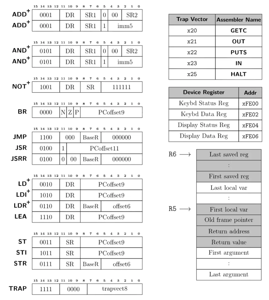
Note: Instructions marked with a + set condition codes, 1 bit each for negative, zero, and positive.
Overall, the architecture is relatively simple and easy to understand. Due to how simple it is though, it can sometimes take many instructions to perform a single operation. For example, there is no subtraction instruction, so it becomes a combination of NOT and ADDs. Also, due to how few bits are in the pc offset of memory-accessing instructions, oftentimes calls will need to be indirect or instructions will need to load values from some predefined global variables. However, I will describe these issues more in detail in later sections.
Note (Lack of compiler)
LC3 does not actually have an official compiler. Now this may sound ridiculous to write a decompiler for an architecture with no compiler (which it kind of is), but it can still work well. However, issues show up especially when it comes to things like the stack and calling convention, since these need to be enforced by the programmer writing the assembly. Overall, this will make edge cases more common, but the goal of this decompiler is not to be perfect, but to demonstrate the decompilation process in LC3.
Example program
As I walk through the steps of the decompiler, I will use the following program as the example input. Here is the intended pseudocode:
int minIndex = 0;
int minValue = ARRAY[0];
for (int i = 1; i < LENGTH; i++) {
if (ARRAY[i] < minValue) {
minValue = ARRAY[i];
minIndex = i;
}
}
mem[mem[RESULT]] = minIndex;And here is the assembly:
AND R0, R0, 0 ; R0 = minIndex = 0
LDI R1, ARRAY ; R1 = minValue = ARRAY[0]
AND R2, R2, 0
ADD R2, R2, 1 ; R2 = i = 1
FORSTART
AND R3, R3, 0
ADD R3, R2, 0 ; R3 = i
LD R4, LENGTH
NOT R4, R4
ADD R4, R4, 1 ; R4 = -length
ADD R3, R3, R4 ; R3 = i - length
BRZP FOREND
LD R3, ARRAY
ADD R3, R3, R2 ; R3 = addr of array[i]
LDR R3, R3, 0 ; R3 = array[i]
AND R4, R4, 0
ADD R4, R4, R1
NOT R4, R4
ADD R4, R4, 1 ; R4 = -minValue
AND R5, R5, 0
ADD R5, R3, R4 ; R5 = array[i] - minValue
BRZP NOTIF
AND R1, R1, 0
ADD R1, R1, R3 ; minValue = array[i]
AND R0, R0, 0
ADD R0, R0, R2 ; minIndex = i
NOTIF
ADD R2, R2, 1
BR FORSTART
FOREND
STI R0, RESULT
HALT
RESULT .fill x4000
ARRAY .fill x5000
LENGTH .fill 5
.end
.orig x4000
ANSWER .blkw 1
.end
.orig x5000
.fill -1
.fill 2
.fill 7
.fill 3
.fill -8
.endStep 1: Disassembly
I wanted the decompiler to take object files as input, so the first step would be to disassemble.
Object files have two sections that I am interested in .TEXT and .SYMBOL. They look like this:
.TEXT
3000
32
5020
A21C
54A0
14A1
....SYMBOL
ADDR | EXT | LABEL
3004 | 0 | FORSTART
3019 | 0 | NOTIF
301B | 0 | FOREND
...These object files are created by the assembler and can then be passed into a simulator. I utilized lc3-ensemble which is a library written by one of the CS 2110 TAs and it can be found here. It has some nice helper functions and structures that make working with the assembly a lot easier.
Now parsing the object file and symbol table is very simple, the only issues arise during disassembly. Since there is no separation between code and data in LC3 object files, there is no trivial way to tell the difference. Luckily, this is not a problem that occurs only in LC3, it is just particularly worse in our situation since there is no notion of a data section, so ALL variables must live among code.
The decompiler design resource has a section on “Identifying Code and Data” which can be found here. Essentially, we will begin at the entrypoint which is passed in as an argument to the decompiler (by default it is 0x3000). Then we disassemble instructions one by one. Some special cases exist:
- If we see a branch, add the destination address to the worklist to visit later and fall through
- If we see a call, add the destination address to a separate call list and fall through
- If we see a return or halt, we end and pop the next item from the worklist
- There are also indirect jumps (JMP reg), in this case the destination is unknown so we treat it like a terminator
- All unvisited addresses are treated as data.
The output of this stage is a map of addresses to instructions/data and a list of function entrypoints identified. For the example program, here is the output of this stage:
Disassembly:
3000: AND R0, R0, #0
3001: LDI R1, #28
3002: AND R2, R2, #0
3003: ADD R2, R2, #1
3004: FORSTART AND R3, R3, #0
3005: ADD R3, R2, #0
3006: LD R4, #24
3007: NOT R4, R4
3008: ADD R4, R4, #1
3009: ADD R3, R3, R4
300A: BRzp #16
300B: LD R3, #18
300C: ADD R3, R3, R2
300D: LDR R3, R3, #0
300E: AND R4, R4, #0
300F: ADD R4, R4, R1
3010: NOT R4, R4
3011: ADD R4, R4, #1
3012: AND R5, R5, #0
3013: ADD R5, R3, R4
3014: BRzp #4
3015: AND R1, R1, #0
3016: ADD R1, R1, R3
3017: AND R0, R0, #0
3018: ADD R0, R0, R2
3019: NOTIF ADD R2, R2, #1
301A: BRnzp #-23
301B: FOREND STI R0, #1
301C: HALT
301D: RESULT JSRR R0
301E: ARRAY AND R0, R0, R0
301F: LENGTH .fill #5
4000: ANSWER .fill #0
5000: .fill #65535
5001: .fill #2
5002: .fill #7
5003: .fill #3
5004: .fill #65528
Identified functions:
3000Step 2: Building the CFG
Now the next step is to create a control flow graph of basic blocks. The decompiler design resource has two relevant sections titled “Basic Blocks” and “Control Flow Graph” which can be found here and here respectively.
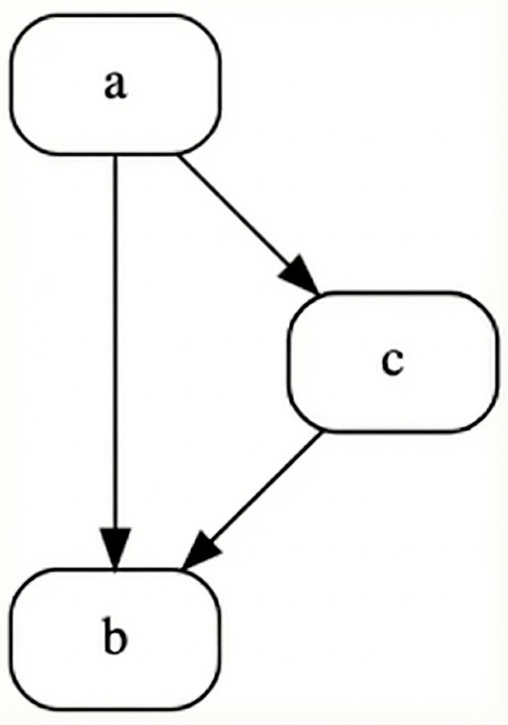
Basic blocks are simply sequences of instructions that we can guarantee can only be entered through the first instruction and exited through the last. To ensure our basic blocks have only one entry and exit, we will terminate a block using the nearest label or branch instruction. We know where labels are from our symbol table and branches can be found simply by looking through the disassembly. We then link predecessors and successors by looking at the last instruction of a block. Unconditional branches will have one target, conditional branches two, and rets/halts/indirect jumps will have none.
One more piece of information that is important to track for our blocks is dominators. This will help us better understand the control flow and detect loops more easily later on. Essentially, block A dominates block B if every path from the entrypoint to block B must pass through block A. An algorithm for computing dominators is also described at the start of the “Loop Analysis” section of the decompiler design resource found here.
Our algorithm begins by initializing the entry block’s dominator set as itself and all other blocks’ sets as every block dominating them. Then, for each non-entry block we update its dominator set to be the intersection of its set and its predecessors’ dominator sets. We repeat this process until no more sets change.
To store all of this information we create a BasicBlock struct:
pub struct BasicBlock {
pub length: u16,
pub preds: Vec<u16>,
pub succs: Vec<u16>,
pub dominators: Vec<u16>,
}Now, we can output a mapping of address to basic blocks that we have found along with their properties. For our example program, the output of this stage is:
Basic blocks:
Block at 3000: length = 4, preds = [], succs = [3004], dominators = [3000]
Block at 3004: length = 7, preds = [3000, 3019], succs = [301B, 300B], dominators = [3000, 3004]
Block at 300B: length = 10, preds = [3004], succs = [3019, 3015], dominators = [3000, 3004, 300B]
Block at 3015: length = 4, preds = [300B], succs = [3019], dominators = [3000, 3004, 300B, 3015]
Block at 3019: length = 2, preds = [300B, 3015], succs = [3004], dominators = [3000, 3004, 300B, 3019]
Block at 301B: length = 2, preds = [3004], succs = [], dominators = [3000, 3004, 301B]Step 3: Control Flow Identification
The next stage is to start identifying higher level control flow structures, namely loops and conditionals. The decompiler design resource does this in the second half of the “Loop Analysis” section found here and the “Creating Statements” section here.
We start by identifying natural loops by detecting back edges in the CFG. Here, back edges are defined as edges where the target block dominates the source block. For each back edge found, we work backwards from the tail and add any blocks that can reach the tail without going through the header, thus adding blocks to the loop body.
For our example program, the output of this stage is:
Natural loops:
Loop 1: header = 3004, blocks = [3019, 3004, 300B, 3015]Next, we improve our natural loops to add more information.
- First, we merge
natural loops with the same header. This allows for the creation of compound
conditions like
while (a && b). - Next, we sort loops from innermost to outermost, so nested loops are handled correctly.
- Finally, we identify key blocks which are the break and continue blocks. A break block is the first successor outside the loop body (the destination of high level break statements) and a continue block is the block containing the back edge (the destination of high level continue statements).
To store this information, we create a new Loop struct:
pub struct Loop {
pub header: u16,
pub blocks: HashSet<u16>,
pub break_block: Option<u16>,
pub continue_block: Option<u16>,
}The output of this stage is a list of Loop objects. For our example program, the output is:
Identified Loop Structures:
Loop 1: header = 3004, blocks = [3019, 3004, 300B, 3015], break_block = Some("301B"), continue_block = Some("3019")Finally, we identify conditionals. We use two main patterns the classic if-else diamond shape and the simple if structure:

The if-else structure in code:
if(expr) if(!expr) {
goto Lfalse
.... ....
goto Lelse }
Lfalse: else {
.... ....
Lelse: }
.... .... And the simple if structure:
if(expr) if(!expr) {
goto Lfalse
.... ....
Lfalse: }These are found easily by iterating through our blocks and analyzing their successors. For example, if a block has two successors and both join to a single block, then it is an if-else structure. To house this information we create a Conditional struct:
pub struct Conditional {
pub kind: ConditionalType,
pub condition_block: u16,
pub true_block: u16,
pub false_block: Option<u16>,
pub join_block: u16,
}For our example program, the output of this step is:
Identified Conditional Structures:
Conditional 1 (If): condition_block = 300B, true_branch = 3015, join_block = 3019Important (Why not structuring?)
At this point in decompilation, we have only identified structures and stored them separately in their respective data structures. There are many reasons for this, but the primary reason is that we need to create the contents of loop/conditional expressions during structuring. For example, even a loop with a simple condition of while (a < b) will require many instructions to compute a - b to set condition codes for the conditional branch. How do we know which instructions are part of this condition and which aren’t? This is what we will address in the next stage before we return to control flow structuring.
Step 4: Liveness and Dataflow Analysis
Onto data flow analysis. The goal here is to start analyzing arithmetic instructions. We will try to remove as many register references as possible and collapse instructions where it is safe to do so. The section “Data Flow Analysis” of the decompiler design resource covers this here.
What we will do is calculate the “livein” and “liveout” sets for each instruction. These are the registers that are alive before executing the instruction and after executing the instruction, respectively. This will be stored as a bit vector where each bit represents a register. We will use this information later to collapse instructions as we will know which registers are not needed later and can be safely inlined or removed.
This process will happen in three phases:
- Compute liveness information for each basic block without considering its relationship to other basic blocks.
Here, we look through each instruction and check what registers are written to (defs) and which registers are read from (uses). Then on the block level, we compute block uses as registers used before being defined in the block and block defs as registers defined anywhere in the block.
Use[B] |= (uses & !block_def)
Def[B] |= defs- Propagate liveness information from each block to all other blocks in the CFG.
Here, we use a fixed-point iteration algorithm to calculate a block’s liveout set as the union of the livein sets of all its successors and a block’s livein set as the union of its block uses and its liveout set minus its block defs.
Out[B] = ∪ In[S] for all successors S
In[B] = Use[B] ∪ (Out[B] - Def[B])- Add information collected from other blocks to each instruction present in a block.
Here, we know which registers are live at the boundaries of each block, but not per instruction. So, we walk backwards through each block and apply block-level liveness information to each instruction with the following algorithm:
live_out[instr] = current_live
live_in[instr] = uses[instr] ∪ (live_out[instr] - defs[instr])
current_live = live_in[instr]The output of this stage is a map of instruction addresses to their use, def, livein, and liveout sets. For our example program, this looks like:
Liveness Analysis:
3000: defs=01, uses=00, in=00, out=01
3001: defs=02, uses=00, in=01, out=03
3002: defs=04, uses=00, in=03, out=07
3003: defs=04, uses=04, in=07, out=07
3004: defs=08, uses=00, in=07, out=07
3005: defs=08, uses=04, in=07, out=0F
3006: defs=10, uses=00, in=0F, out=1F
3007: defs=10, uses=10, in=1F, out=1F
3008: defs=10, uses=10, in=1F, out=1F
3009: defs=08, uses=18, in=1F, out=07
300A: defs=00, uses=00, in=07, out=07
300B: defs=08, uses=00, in=07, out=0F
300C: defs=08, uses=0C, in=0F, out=0F
300D: defs=08, uses=08, in=0F, out=0F
300E: defs=10, uses=00, in=0F, out=1F
300F: defs=10, uses=12, in=1F, out=1F
3010: defs=10, uses=10, in=1F, out=1F
3011: defs=10, uses=10, in=1F, out=1F
3012: defs=20, uses=00, in=1F, out=1F
3013: defs=20, uses=18, in=1F, out=0F
3014: defs=00, uses=00, in=0F, out=0F
3015: defs=02, uses=00, in=0C, out=0E
3016: defs=02, uses=0A, in=0E, out=06
3017: defs=01, uses=00, in=06, out=07
3018: defs=01, uses=05, in=07, out=07
3019: defs=04, uses=04, in=07, out=07
301A: defs=00, uses=00, in=07, out=07
301B: defs=00, uses=01, in=01, out=00
301C: defs=00, uses=00, in=00, out=00Step 5: IR Lifting and Expression Propagation
Now that we have liveness information, we can safely inline instructions where possible. In the process, we will also lift instructions into an IR that is mostly composed of Assigns, Stores, Gotos, and Expressions. This step is covered in the “Expressions Propagation” section of the decompiler design resource found here.
Essentially, we will go through our assignment instructions one by one and add them as “pending assignments”. When the assigned register is later used, if it is dead after use we can inline the assignment. Otherwise, we must flush the assignment and use a register reference where it is used.
Once this is complete, we will have many inlined expressions together for individual IR assignments. This lets us collapse them with some standard identities. We run this in a fixed-point loop until no more simplifications can be made.
| Pattern | Simplification |
|---|---|
| Not(Not(x)) | x |
| And(x, 0) | 0 |
| Add(Not(x), 1) | Neg(x) |
| … | … |
We also do a quick pass to attach condition expressions to Goto statements. Similar to how we collapse assignments, if we see a register is dead after its assignment right before a goto, we know it was only used to set condition codes. So, we simply attach the condition expression to the goto statement and remove the assignment.
The output of this stage is a map of addresses to IR assignments, categorized within their basic blocks. For our example program, here is the output IR before and after collapsing assignments:
Expressions:
Block 3000:
3000: Assign(0, And(Register(0), Immediate(0x0)))
3001: Assign(1, Load(Load(Immediate(0x301E))))
3003: Assign(2, Add(And(Register(2), Immediate(0x0)), Immediate(0x1)))
Block 3004:
3009: Assign(3, Add(Add(Register(2), Immediate(0x0)), Add(Not(Load(Immediate(0x301F))), Immediate(0x1))))
300A: Goto(None, 0x3, 0x301B)
Block 300B:
300D: Assign(3, Load(Add(Add(Load(Immediate(0x301E)), Register(2)), Immediate(0x0))))
3013: Assign(5, Add(Register(3), Add(Not(Add(And(Register(4), Immediate(0x0)), Register(1))), Immediate(0x1))))
3014: Goto(None, 0x3, 0x3019)
Block 3015:
3016: Assign(1, Add(And(Register(1), Immediate(0x0)), Register(3)))
3018: Assign(0, Add(And(Register(0), Immediate(0x0)), Register(2)))
Block 3019:
3019: Assign(2, Add(Register(2), Immediate(0x1)))
301A: Goto(None, 0x7, 0x3004)
Block 301B:
301B: Store(Load(Immediate(0x301D)), Register(0))Collapsed Expressions:
Block 3000:
3000: Assign(0, Immediate(0x0))
3001: Assign(1, Load(Load(Immediate(0x301E))))
3003: Assign(2, Immediate(0x1))
Block 3004:
300A: Goto(Some(Sub(Register(2), Load(Immediate(0x301F)))), 0x3, 0x301B)
Block 300B:
300D: Assign(3, Load(Add(Load(Immediate(0x301E)), Register(2))))
3014: Goto(Some(Sub(Register(3), Register(1))), 0x3, 0x3019)
Block 3015:
3016: Assign(1, Register(3))
3018: Assign(0, Register(2))
Block 3019:
3019: Assign(2, Add(Register(2), Immediate(0x1)))
301A: Goto(None, 0x7, 0x3004)
Block 301B:
301B: Store(Load(Immediate(0x301D)), Register(0))Step 6: Control Flow Structuring
Now we can return to creating control flow structures we identified earlier. This is covered in the “Creating Statements” section of the decompiler design resource found here.
I broke this process down into five steps:
- Merge Compound Conditions
This is done first, since it is easier to detect these patterns before any loop structures are fully created yet. This way once we have created a loop with an expression, we can be relatively confident there are no other checks or boolean expressions.
I’m not sure if there’s a sophisticated algorithm for this, but I just looked for consecutive gotos with the same target address. Most of this came from simply testing examples and trying to detect the most common patterns. By the end, any adjacent conditionals are combined together with a LogicalOr expression type.
For example, patterns like:
if (cond1) goto L_false;
if (cond2) goto L_false;
// ... true path ...Become: if (cond1 || cond2) goto L_false
- Structure Loops
Now it is time to create loop structures using the following steps:
- Use the already computed natural loops and for each one create a DoWhile statement in the IR
- Take all blocks in the loop body and move them into the statement
- Find the goto that exits to the break block and negate it to create the condition
- Remove this goto since it is now implicit
- Any gotos with a destination of the break block become break statements
- Any gotos with a destination of the continue block become continue statements
The DoWhile statement in the IR is defined as:
DoWhile(Option<Expr>, u8, HashMap<u16, Vec<IRStmt>>)Where the Option<Expr> is the condition, the u8 is the condition code, and
the HashMap<u16, Vec<IRStmt>> is the loop body.
- Structure Conditionals
Now we can create if/if-else statements. Most of the work here was already done in the identification step. For if-else patterns, we extract the true and false blocks and put it in our IR statements. For simple if patterns, we just extract the true block. This process also happens recursively to descend into any loop bodies first.
The If statement in the IR is defiend as:
If(Option<Expr>, u8, Vec<IRStmt>, Option<Vec<IRStmt>>)Where the Option<Expr> is the condition, the u8 is the condition code, the
Vec<IRStmt> is the true block, and the Option<Vec<IRStmt>> is the false
block which is None in the simple if case.
- Refine Loops
Now in our loop structuring we assumed all loops are do whiles by default. This step will create while loops and for loops where appropriate. First we convert do while loops to while loops based on the following pattern:
if(expr) while(expr) {
goto Lbreak;
do {
.... ....
} while(expr); }
Lbreak:
.... ....Note (Why conditionals were structured first)
Hopefully this makes it clear why we structured conditionals before refining our loops. It becomes much easier to detect the while loop pattern as an if above a do while loop. Both check the same condition.
Then we convert while loops to for loops based on the following pattern. An initialization statement must be present in the predecessor block, that same variable must be used in the condition, and that variable is also incremented at the end of the loop body.
v = init_expr
while(expr comparing v) { for(v = init_expr; expr comparing v; v = incr) {
....
Lcontinue:
v = incr // e.g. v += 1
} }
....- Cleanup Control Flow
One last step is to remove certain redundant statements. There will often be continues at the end of a loop body that are not needed or unnecessary gotos that fall through a conditional. These become easier to detect once our loops are in their fully structured form (while, do while, for).
The output of this stage is similar to our collapsed expression from the previous stage, but now certain statements are nested inside of control flow structures and rearranged. For our example program, this looks like:
Structured Control Flow:
Block 3000:
3000: Assign(0, Immediate(0x0))
3001: Assign(1, Load(Load(Immediate(0x301E))))
Block 3004:
3004: For(Assign(2, Immediate(0x1)), Some(Sub(Register(2), Load(Immediate(0x301F)))), 0x4, Assign(2, Add(Register(2), Immediate(0x1))), {
Block 3004:
Block 300B:
Assign(3, Load(Add(Load(Immediate(0x301E)), Register(2))))
If(Some(Sub(Register(3), Register(1))), 0x4, {
Assign(1, Register(3))
Assign(0, Register(2))
})
Block 3019:
})
Block 301B:
301B: Store(Load(Immediate(0x301D)), Register(0))Step 7: Handling Calling Convention
Before we finish, we need to take one last detour regarding calling conventions. I ran into some trouble here since not all test programs I had followed this convention strictly, especially the simpler tests. I ended up making this an optional argument that can be passed into the decompiler.
There are two main cases that we have to handle for the caller and the callee.
- Callee
There are three main issues here that make the current decompilation quite ugly for functions being called.
- Prologue: There are many instructions involved in setting up the stack frame and saving registers. We essentially look for the last instruction that saves a general purpose register and clear all instructions before it.
- Epilogue: There is also callee teardown. This one is easier to detect since
the first instruction always saves the return value at some offset from R5. We
simply remember which register is used for the return value, remove all
instructions after it, and insert a single
return varXstatement. - Parameter Passing: Lastly, anytime function parameters are used they are
loaded from R5+4, R5+5, etc. We simply replace these with more recognizable
paramXnames where X is the parameter’s index.
- Caller
In LC3 when a function is called, first parameters are pushed onto the stack,
then the call is executed, and then the return value is popped off the stack and
the stack pointer is restored. Ideally, we want calls to be condensed to just
one instruction like varX = func(param0, param1).
Push sequences subtract from the stack pointer and store, so the parameters pushed are stored and these instructions are removed. After a function call, we simply look for the load instruction that grabs the return value and the add that fixes the stack pointer. We track the register storing the return value and remove these instructions.
Here is an example of a fibonacci function implementation run with and without the calling convention argument:
Structured Control Flow:
Block 4000:
4001: Assign(6, Add(Register(6), Immediate(0xFFFE)))
4002: Store(Register(6), Register(7))
4003: Assign(6, Add(Register(6), Immediate(0xFFFF)))
4004: Store(Register(6), Register(5))
4007: Assign(6, Add(Register(6), Immediate(0xFFFD)))
4008: Store(Register(6), Register(0))
4009: Assign(6, Add(Register(6), Immediate(0xFFFF)))
400A: Store(Register(6), Register(1))
400B: Assign(6, Add(Register(6), Immediate(0xFFFF)))
400C: Store(Register(6), Register(2))
400D: Assign(6, Add(Register(6), Immediate(0xFFFF)))
400E: Store(Register(6), Register(3))
400F: Assign(0, Load(Add(Add(Register(6), Immediate(0xFFFF)), Immediate(0x4))))
4010: Assign(2, Add(Register(0), Immediate(0xFFFF)))
4011: If(Some(Register(2)), 0x1, {
Assign(0, Register(2))
Assign(6, Add(Register(6), Immediate(0xFFFF)))
Store(Register(6), Register(0))
Call(Immediate(0x4000))
Assign(3, Load(Register(6)))
Assign(6, Add(Register(6), Immediate(0x1)))
Store(Register(6), Add(Register(0), Immediate(0xFFFF)))
Call(Immediate(0x4000))
Assign(6, Add(Register(6), Immediate(0x2)))
Assign(1, Add(Register(3), Load(Register(6))))
} else {
Assign(1, Register(0))
})
Block 4023:
4023: Store(Add(Register(5), Immediate(0x3)), Register(1))
4024: Assign(3, Load(Register(6)))
4025: Assign(6, Add(Register(6), Immediate(0x1)))
4026: Assign(2, Load(Register(6)))
4027: Assign(6, Add(Register(6), Immediate(0x1)))
4028: Assign(1, Load(Register(6)))
4029: Assign(6, Add(Register(6), Immediate(0x1)))
402A: Assign(0, Load(Register(6)))
402C: Assign(6, Add(Register(6), Immediate(0x3)))
402D: Assign(5, Load(Register(6)))
402E: Assign(6, Add(Register(6), Immediate(0x1)))
402F: Assign(7, Load(Register(6)))
4030: Assign(6, Add(Register(6), Immediate(0x1)))
4031: ReturnStructured Control Flow:
Block 4000:
400F: Assign(0, Param(0))
4010: Assign(2, Add(Register(0), Immediate(0xFFFF)))
4011: If(Some(Register(2)), 0x1, {
Assign(0, Register(2))
Assign(3, CallExpr(Immediate(0x4000), Register(0)))
Assign(1, Add(Register(3), CallExpr(Immediate(0x4000), Add(Register(0), Immediate(0xFFFF)))))
} else {
Assign(1, Register(0))
})
Block 4023:
4031: Return(Register(1))Step 8: Linearization and Code Output
We are so close to the end, but our IR at this point is stored as map of addresses to IRStmts. We need to remove any notion of addresses and blocks to output a clean vector of statements.
Here, we simply sort blocks by address and output statments one by one. We do need to keep track of any gotos that we were not able to turn into some control flow statement. In this case, we preserve its destination label and output it at the right address. Finally, we also do this recursively to properly handle nested loops and conditionals.
After linearization is also a good time to do any miscellaneous cleanup. If certain control flow structures were hard to detect earlier or if there are any unnecessary labels we can remove them now.
This will output a vector of linearized code. For our example program, this looks like:
Linearized Code:
Assign(0, Immediate(0x0))
Assign(1, Load(Load(Immediate(0x301E))))
For(Assign(2, Immediate(0x1)), Some(Sub(Register(2), Load(Immediate(0x301F)))), 0x4, Assign(2, Add(Register(2), Immediate(0x1))), {
Assign(3, Load(Add(Load(Immediate(0x301E)), Register(2))))
If(Some(Sub(Register(3), Register(1))), 0x4, {
Assign(1, Register(3))
Assign(0, Register(2))
})
})
Store(Load(Immediate(0x301D)), Register(0))Finally, we convert these statements one by one to C-like syntax. Registers become varX where X is the register number, arithmetic operations become their respective symbols, accessing memory becomes pointer dereferencing, etc. Also, loop headers and conditionals up until now still stored their condition code number, so we need to convert the bits of NZP to their respective comparison symbols. This process is partly up to personal preference, so I won’t go into detail about it here.
One last step to make our code output even better for LC3 is to use the symbol table we extracted from the object file earlier. Any references that load, store, or call some address present in the symbol table can be resolved to their respective names.
The output is simply the string containing the code. For our example program, it looks like:
Generated C-Like Code:
var0 = 0;
var1 = *(*ARRAY);
for (var2 = 1; var2 < *LENGTH; var2++) {
var3 = *(*ARRAY + var2);
if (var3 < var1) {
var1 = var3;
var0 = var2;
}
}
**RESULT = var0;Conclusion
If we compare the output to the intended pseudocode, we can see it is nearly the same.
int minIndex = 0;
int minValue = ARRAY[0];
for (int i = 1; i < LENGTH; i++) {
if (ARRAY[i] < minValue) {
minValue = ARRAY[i];
minIndex = i;
}
}
mem[mem[RESULT]] = minIndex;This decompiler is by no means perfect. Ideally, many of these stages would be repeated since they usually make the final result much more accurate. This is mentioned in the “Standard Decompiler Architecture” section of the decompiler design resource found here where it mentions “We’ll see in the advanced section that it is not possible to perform advanced decompilation in a single pass over the input program. The use of multiple passes may make some analysis more complicated, but it will give much better results.”
The biggest issues I am aware of are that any indirect jumps or calls are not handled at all. The calling convention is also handled very naively, so local variables are not detected. Some code could also be better optimized to remove unnecessary assignments.
Overall though, I’m very satisfied with the result and think this project helped me understand the decompilation process much better which oftentimes feels very black boxy. If you read this far thanks for sticking around and I hope you learned something new!